Most monitors are capable of displaying RGB values in the range of $[0, 255]$ . However, in real life, there is no limit on the amount of light 'energy' incident on a point. Most renderers output linear radiance values in $[0, \infty)$ , which needs to be mapped into a viewable range. Those radiance values are described as High Dynamic Range (HDR), because they are unlimited, and the viewable target range is described as Low Dynamic Range (LDR), because there is a fixed limit of 255. Put simply, tone mapping is the process of mapping HDR values in $[0, \infty)$ into LDR values (e.g values in $[0, 255]$ or $[0.0, 1.0]$ ).

A tone mapping operator (TMO) is essentially just a function which maps an input color (e.g an RGB triple) to an output color:

At this point you might be a little confused as to why you've never had to think about tone mapping inside your program. If you're using an API like OpenGL, your radiance values are probably just being clamped by the implementation to $[0.0, 1.0]$ in the final framebuffer. This is essentially a trivial tone mapping operator:

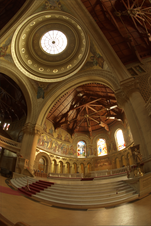
This TMO, as you might guess, is quite flawed. Here's what it looks like when we apply this TMO to the memorial scene (the HDR scene file can be downloaded here):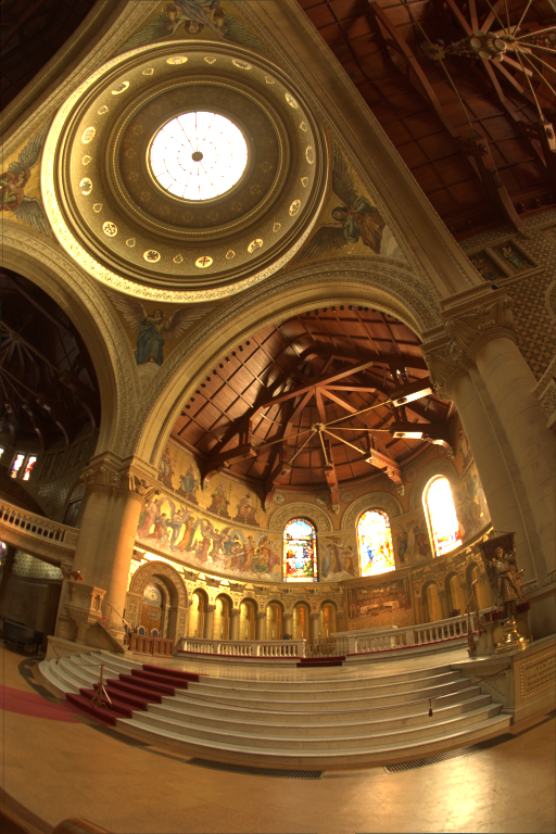

High radiance values are being completely lost beyond a certain point. This results in the white areas (like the middle stained glass window) looking completely 'blown out'. For this particular scene it's not too bad because most of the radiance values are in $[0.0, 1.0]$ already, but for a brighter outdoors scene it would look a lot worse. You could alleviate the issue somewhat by dividing the input color by some value before clamping:

However, as it turns out, we don't really want a linear relationship between input and output color. Human color perception is very non-linear - the difference between 1 light source and 2 light sources illuminating a point appears much greater than the difference between 100 light sources and 101 light sources. Non-linear TMOs are potentially able to reproduce images which can convey more detail to our eyes. Floats actually work great for storing HDR values for this exact reason - they have higher precision nearer zero, and lower precision as their value increases towards infinity.

The rest of this guide will explore a few simple tone mapping operators, as well as some underlying theory which should help you research the topic further.

Reinhard

This is one of the simplest and most common TMOs, described by Reinhard et al. in this paper. Simply put, it is:

(Note that this isn't exactly what Reinhard is proposing in his paper, but more on that further down.)

This is mathematically guaranteed to produce a value in $[0.0, 1.0]$ . By differentiating, you can see that $C_{\mathrm{out}}$ has an inverse-square falloff (e.g a radiance value of 4 results in something which is only 1.2 times as bright as a radiance value of 2).

In C++:

vec3 reinhard(vec3 v)
{
    return v / (1.0f + v);
}

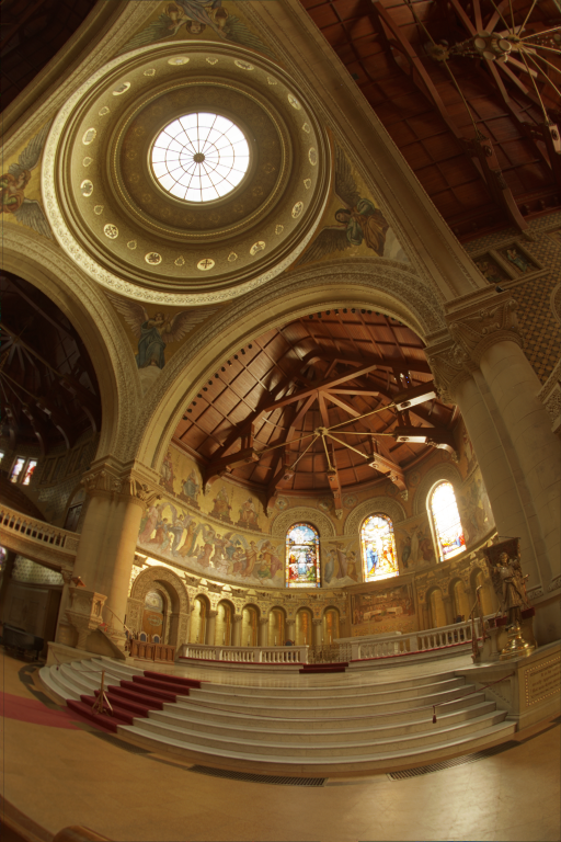
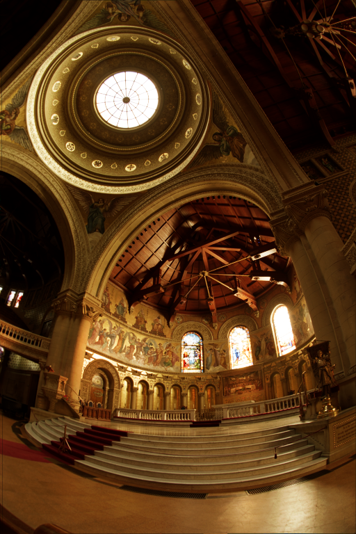
Compare this image to the previous 'clamp' TMO. Reinhard looks much more grey-ish, and the whites are less blown out (more detail is noticeable in the middle stained glass window).

Extended Reinhard

The problem with the 'simple' Reinhard TMO is that it doesn't necessarily make good use of the full Low Dynamic Range. If our max scene radiance happened to be $(1.0, 1.0, 1.0)$ then the resulting maximum brightness would only be $(0.5, 0.5, 0.5)$ - only half of the available range. Fortunately, the paper by Reinhard presents a way to scale and make use of the full range:

where $C_{\mathrm{white}}$ is the biggest radiance value in the scene. Now, our biggest radiance value will get mapped to $(1.0, 1.0, 1.0)$ , using the full LDR.

(Note that you can also just set $C_\mathrm{white}$ to a value lower than the maximum radiance, which will ensure that anything higher gets mapped to $(1.0, 1.0, 1.0)$ - for this reason it is sometimes referred to as the 'white point'.)

In C++:

vec3 reinhard_extended(vec3 v, float max_white)
{
    vec3 numerator = v * (1.0f + (v / vec3(max_white * max_white)));
    return numerator / (1.0f + v);
}

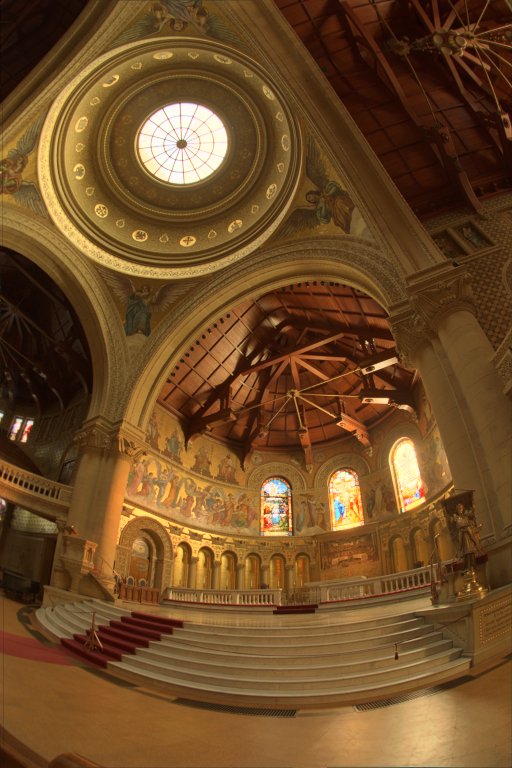
If we just set our max scene radiance as the white point, this TMO appears almost exactly the same as the simple reinhard operator. That's because the max radiance for this scene is 622, and $\frac{622}{1+622} \approx 0.998$ , so the difference between the extended and the simple variants in this case is imperceptible - simple reinhard was already making full use of the low dynamic range. If we used a different white point, the TMO would look noticeably different.

Luminance and Color Theory

Okay, so I must admit that I've lied to you slightly. Reinhard's formulas actually operate on a thing called luminance rather than operating on RGB-triples as I implied. Luminance is a single scalar value which measures how bright we view something. It may not be obvious, but for example we perceive green as much brighter than blue. In other words, $(0.0, 0.7, 0.0)$ appears much brighter than $(0.0, 0.0, 0.7)$ .

Converting a linear RGB triple to a luminance value is easy:

So far we've effectively been applying our TMOs to each RGB channel individually. However this can cause a 'shift' in hue or saturation which can significantly change the color appearance.

Instead, what Reinhard's formula entails is to convert our linear RGB radiance to luminance, apply tone mapping the luminance, then somehow scale our RGB value by the new luminance. The simplest way of doing that final scaling is:

In C++:

float luminance(vec3 v)
{
    return dot(v, vec3(0.2126f, 0.7152f, 0.0722f));
}

vec3 change_luminance(vec3 c_in, float l_out)
{
    float l_in = luminance(c_in);
    return c_in * (l_out / l_in);
}

Two other more complex luminance-adjusting methods are discussed in a paper by Mantiuk et al., but the simple method is perfectly acceptable.

Don't confuse luminance with luma - luma is the equivalent of the luminance computed from an sRGB pixel (i.e gamma-corrected). The coefficients used to convert to luma are the same as luminance, they just operate on sRGB components instead. See Wikipedia for more details.

Note that the hue / saturation preservation which results from this method isn't always desirable. Reinhard tone mapping in particular was created with the intention of being applied to luminance only, so it looks much better when this is done (see the following section for details on that). Other tone mapping curves look better when applied to RGB components separately.

Reinhard was on the wrong track in applying his tone mapping curve to luminance; his curve was inspired by film, but film curves are applied to each color channel separately. And that is a good thing - [...] the "hue and saturation shifts" (really mostly saturation shifts) resulting from applying nonlinear curves per channel are an important feature, not a bug.

-- Naty Hoffman, co-author of Real Time Rendering

Extended Reinhard (Luminance Tone Map)

Let's apply the extended Reinhard TMO to luminance only:

vec3 reinhard_extended_luminance(vec3 v, float max_white_l)
{
    float l_old = luminance(v);
    float numerator = l_old * (1.0f + (l_old / (max_white_l * max_white_l)));
    float l_new = numerator / (1.0f + l_old);
    return change_luminance(v, l_new);
}

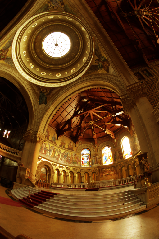
Here's the difference it makes - the stained glass windows and the column on the left are noticeably more orange and less 'washed out' in the luminance mapped version:

Note that in fact with Reinhard, the luminance calculation can be simplified somewhat:

Hence

Reinhard-Jodie

You aren't necessarily forced to choose between tone mapping RGB individually and tone mapping luminance. Here's one such Reinhard variant by shadertoy user Jodie which does that:

vec3 reinhard_jodie(vec3 v)
{
    float l = luminance(v);
    vec3 tv = v / (1.0f + v);
    return lerp(v / (1.0f + l), tv, tv);
}

The difference between this and the luminance-only tone map is barely noticeable in this scene (you can see that the stain glass windows are slightly less orange), but in other scenes (especially those with colored lights) the difference is more obvious. Note that there's also no way to set the white point with this TMO, but you could add a way yourself.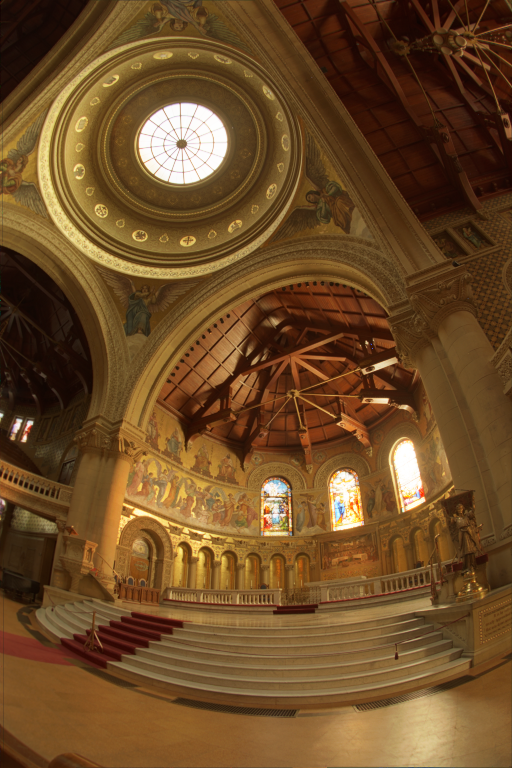

Filmic Tone Mapping Operators

So-called 'filmic' TMOs are designed to emulate real film. Other than that, their defining feature is the distinctive 'toe' at the bottom end of the curve (radiance is on the $x$ -axis, final pixel brightness is on the $y$ -axi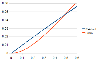s):

Note that the other end of the tone mapping curve is usually described as the 'shoulder'.

Uncharted 2

A popular TMO for real-time graphics is the Uncharted 2 TMO devised by John Hable (sometimes known as 'Hable Tone Mapping' or 'Hable Filmic' etc). It has some parameters which can be tweaked, but the basic operator is given by the following code:

vec3 uncharted2_tonemap_partial(vec3 x)
{
    float A = 0.15f;
    float B = 0.50f;
    float C = 0.10f;
    float D = 0.20f;
    float E = 0.02f;
    float F = 0.30f;
    return ((x*(A*x+C*B)+D*E)/(x*(A*x+B)+D*F))-E/F;
}

vec3 uncharted2_filmic(vec3 v)
{
    float exposure_bias = 2.0f;
    vec3 curr = uncharted2_tonemap_partial(v * exposure_bias);

    vec3 W = vec3(11.2f);
    vec3 white_scale = vec3(1.0f) / uncharted2_tonemap_partial(W);
    return curr * white_scale;
}

For some further reading, see John Hable's blog post about creating an improved curve which offers more intuitive controls.

ACES

Another popular filmic tone mapping curve is ACES (Academy Color Encoding System). This is the default TMO used by Unreal Engine 4 so would be a perfectly good choice to use in your own real-time engine. The TMO curve is calculated through a couple of matrix transformations and formulae adapted from Stephen Hill's fit, shown below:

static const std::array<vec3, 3> aces_input_matrix =
{
    vec3(0.59719f, 0.35458f, 0.04823f),
    vec3(0.07600f, 0.90834f, 0.01566f),
    vec3(0.02840f, 0.13383f, 0.83777f)
};

static const std::array<vec3, 3> aces_output_matrix =
{
    vec3( 1.60475f, -0.53108f, -0.07367f),
    vec3(-0.10208f,  1.10813f, -0.00605f),
    vec3(-0.00327f, -0.07276f,  1.07602f)
};

vec3 mul(const std::array<vec3, 3>& m, const vec3& v)
{
    float x = m[0][0] * v[0] + m[0][1] * v[1] + m[0][2] * v[2];
    float y = m[1][0] * v[0] + m[1][1] * v[1] + m[1][2] * v[2];
    float z = m[2][0] * v[0] + m[2][1] * v[1] + m[2][2] * v[2];
    return vec3(x, y, z);
}

vec3 rtt_and_odt_fit(vec3 v)
{
    vec3 a = v * (v + 0.0245786f) - 0.000090537f;
    vec3 b = v * (0.983729f * v + 0.4329510f) + 0.238081f;
    return a / b;
}

vec3 aces_fitted(vec3 v)
{
    v = mul(aces_input_matrix, v);
    v = rtt_and_odt_fit(v);
    return mul(aces_output_matrix, v);
}

You can also use this approximated ACES fit by Krzysztof Narkowicz for something a bit more performant. Note that this approximation oversaturates bright colors slightly compared to the better fit (you can see that in the middle stained glass window).

vec3 aces_approx(vec3 v)
{
    v *= 0.6f;
    float a = 2.51f;
    float b = 0.03f;
    float c = 2.43f;
    float d = 0.59f;
    float e = 0.14f;
    return clamp((v*(a*v+b))/(v*(c*v+d)+e), 0.0f, 1.0f);
}

Real Camera Response Functions

Sometimes it might be desireable to exactly reproduce the 'tone mapping' response of a real camera. Fortunately, the University of Columbia has released a database of camera response functions which we can use for this purpose. Each camera response curve has two axes: irradiance (essentially the energy coming into the camera) and intensity (essentially the value of color component at that point on the film).

Since irradiance is the input and intensity is the output, you can visualise irradiance and intensity on the $x$ and $y$ axes respectively. The data given to us has the points on both axes normalized into the range $[0.0, 1.0]$ . For intensity, this is exactly what we want, as we can just scale the output by 256 to get the corresponding 8-bit color component. For irradiance, we will need to decide the 'width' of the curve. Since the point with the largest $x$ value is $(1.0, 1.0)$ , if we stretch this curve horizontally by a factor of $a$ then the new furthest point will be $(a, 1.0)$ . We can map any irradiance value greater than $a$ to $1.0$ and hence we can effectively control the white point by stretching or squashing the irradiance axis. Instead of 'white point', we'll call this parameter 'ISO' which mimics the function of the ISO setting on a real-world camera.

The data is given as two associative arrays. Given a irradiance value in $[0.0, 1.0]$ we need to find the index into the irradiance array (ideally using a binary search). Then, we can compute the output value by using the index we got from that binary search to look up the intensity value from the intensity array. We'll repeat this procedure for each RGB channel individually to compute the final color.

For real-time graphics you might want to find a way to bake a LUT instead of doing a relatively expensive binary search.

float camera_get_intensity(float f, float iso)
{
    f = clamp(f, 0.0f, iso); // Clamp to [0.0, iso]
    f /= iso; // Convert to [0.0, 1.0]

    // Returns 1.0 if the index is out-of-bounds
    auto get_or_one = [](const auto& arr, size_t index)
    {
        return index < arr.size() ? arr[index] : 1.0;
    };

    // std::upper_bound uses a binary search to find the position of f in camera_irradiance
    auto upper = std::upper_bound(camera_irradiance.begin(), camera_irradiance.end(), f);
    size_t idx = std::distance(camera_irradiance.begin(), upper);

    double low_irradiance = camera_irradiance[idx];
    double high_irradiance = get_or_one(camera_irradiance, idx + 1);
    double lerp_param = (f - low_irradiance) / (high_irradiance - low_irradiance);

    double low_val = camera_intensity[idx];
    double high_val = get_or_one(camera_intensity, idx + 1);

    // Lerping isn't really necessary for RGB8 (as the curve is sampled with 1024 points)
    return clamp(lerp((float)low_val, (float)high_val, (float)lerp_param), 0.0f, 1.0f);
}

vec3 camera_tonemap(vec3 v, float iso)
{
    float r = camera_get_intensity(v.r(), iso);
    float g = camera_get_intensity(v.g(), iso);
    float b = camera_get_intensity(v.b(), iso);
    return vec3(r, g, b);
}

This method is available as an option in Indigo Renderer, for the curious.

Local Tone Mapping Operators

So far, all the TMOs I've discussed have been global tone mapping operators. This means that the computation they do is only based on the input radiance value and global image parameters like the average luminance. Tone mapping operators which are a function of position are known as local tone mapping operators. These are generally far more expensive and hence unsuitable for real time graphics - yet widely used in digital photography. Local TMOs can also give strange results when applied to video.

One local tone mapping operator is described in the same paper by Reinhard et al. - it involves a digital simulation of a process known as 'dodging and burning' in real photography, which essentially applies different exposure to different regions of the image, often resulting in more detailed images than global tone mapping operators are able to produce.

Conclusion

Hopefully this guide was instructive. I've placed a grid of all TMOs used here for comparison, but keep in mind that these can be adjusted in certain ways through exposure or other parameters, so this isn't entirely a fair comparison.

Further Reading

• High Dynamic Range Imaging Book, R. Mantiuk et al.
• Filmic Worlds Blog - John Hable
• Tone Mapping (slides) - R. Mantiuk
• Dynamic Range, Exposure and Tone Mapping - Seena Burns

Appendix

The full source code for this post can be found on my GitHub. For the vec3 class, I'm using a slightly modified version of the one found in Shirley's 'Ray Tracing in One Weekend' book.

This guide was initially created by me for the Graphics Programming Discord Resources.